
Depletion approximation
The depletion approximation provides an analytical - or semi-analytical
- solution to the Poisson-drift-diffusion equations described in the
previous section applied to simple PN homojunction solar cells.
Historically, it has been used extensively to model solar cells and it
is still valid, to a large extent, for traditional PN junctions. More
importantly, it requires less input parameters than the PDD solver and
these can be easily related to macroscopic measurable quantities, like
mobility or diffusion lengths. The DA model is based on the assumption
that around the junction between the P and N regions, there are no free
carriers and therefore all the electric field is due to the fixed,
ionized dopants. This “depletion” of free carriers reaches a certain
depth towards the N and P sides; beyond this region, free and fixed
carriers of opposite charges balance and the regions are neutral. Under
these conditions, Poisson’s equation decouples from the drift and
diffusion equations and it can be solved analytically for each region.
For example, for a PN junction with the interface between the two
regions at  , the solution to Poisson’s equation will be:
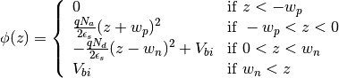
where  and
and  are the extensions of the depletion
region towards the N and P sides, respectively, and can be found by the
requirement that the electric field
are the extensions of the depletion
region towards the N and P sides, respectively, and can be found by the
requirement that the electric field  and the potential
 need to be continuous at .
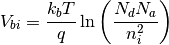
  is the
built-in voltage, which can be expressed in terms of the doping
concentration on each side,
is the
built-in voltage, which can be expressed in terms of the doping
concentration on each side,  and
and  , and the
intrinsic carrier concentration in the material,
, and the
intrinsic carrier concentration in the material,  :
:
Another consequence of the depletion approximation is that the
quasi-Fermi level energies are constant throughout the corresponding
neutral regions and also constant in the depletion region, where their
separation is equal to the external bias  . Based on these
assumptions, the drift-diffusion equations
simplify and an analytical expression can be found for the dependence of
the recombination and generation currents on the applied voltage. A full
derivation of these expressions is included in
Nelson (2003) ([1]).
. Based on these
assumptions, the drift-diffusion equations
simplify and an analytical expression can be found for the dependence of
the recombination and generation currents on the applied voltage. A full
derivation of these expressions is included in
Nelson (2003) ([1]).
Solcore’s implementation of the depletion approximation includes two modifications to the basic equations. The first one is allowing for an intrinsic region to be included between the P and N regions to form a PIN junction. For low injection conditions (low illumination or low bias) this situation can be treated as described before, simply considering that the depletion region is now widened by the thickness of the intrinsic region. Currently, no low doping level is allowed for this region.
The second modification is related to the generation profile, which in
the equations provided by Nelson is given by the BL law
which has an explicit dependence on  and results in analytic
expressions for the current densities. In Solcore, we integrate the
expressions for the drift-diffusion equations under the depletion
approximation numerically or by using the Green’s function method to allow
for an arbitrary generation profile calculated with any of the optical
solvers. It should be noted that although the equations
are integrated numerically this will not be a self-consistent solution of the
Poisson-drift-diffusion equations, as is achieved by the PDD solver.
and results in analytic
expressions for the current densities. In Solcore, we integrate the
expressions for the drift-diffusion equations under the depletion
approximation numerically or by using the Green’s function method to allow
for an arbitrary generation profile calculated with any of the optical
solvers. It should be noted that although the equations
are integrated numerically this will not be a self-consistent solution of the
Poisson-drift-diffusion equations, as is achieved by the PDD solver.
Detailed balance functions
-
solcore.analytic_solar_cells.depletion_approximation.identify_parameters(junction, T, pRegion, nRegion, iRegion)[source]
-
solcore.analytic_solar_cells.depletion_approximation.iv_depletion(junction, options)[source]¶ Calculates the IV curve of a junction object using the depletion approximation as described in J. Nelson, “The Physics of Solar Cells”, Imperial College Press (2003). The junction is then updated with an “iv” function that calculates the IV curve at any voltage.
Parameters: - junction – A junction object.
- options – Solver options.
Returns: None.
-
solcore.analytic_solar_cells.depletion_approximation.get_j_dark(x, w, l, s, d, V, minority, T)[source]¶ Parameters: - x – width of top junction
- w – depletion width in top junction
- l – diffusion length
- s – surface recombination velocity
- d – diffusion coefficient
- V – voltage
- minority – minority carrier density
- T – Temperature
Returns: J_top_dark
-
solcore.analytic_solar_cells.depletion_approximation.get_Jsrh(ni, V, Vbi, tp, tn, w, kbT, dEt=0)[source]
-
solcore.analytic_solar_cells.depletion_approximation.forward(ni, V, Vbi, tp, tn, w, kbT, dEt=0)[source]¶ Equation 27 of Sah’s paper. Strictly speaking, it is not valid for intermediate negative bias.
-
solcore.analytic_solar_cells.depletion_approximation.factor(V, Vbi, tp, tn, kbT, dEt=0)[source]¶ The integral of Eq. 27 in Sah’s paper. While it is coninuum (in principle) it has to be done in two parts. (or three)
-
solcore.analytic_solar_cells.depletion_approximation.get_J_sc_diffusion(xa, xb, g, D, L, y0, S, wl, ph, side='top')[source]¶ Parameters: - xa –
- xb –
- g –
- D –
- L –
- y0 –
- S –
- wl –
- ph –
- side –
Returns: out
-
solcore.analytic_solar_cells.depletion_approximation.get_J_sc_diffusion_green(xa, xb, g, D, L, y0, S, ph, side='top')[source]¶ Computes the derivative of the minority carrier concentration at the edge of the junction by approximating the convolution integral resulting from applying the Green’s function method to the drift-diffusion equation.
Parameters: - xa – Coordinate at the start the junction.
- xb – Coordinate at the end the junction.
- g – Carrier generation rate at point x (expected as function).
- D – Diffusion constant.
- L – Diffusion length.
- y0 – Carrier equilibrium density.
- S – Surface recombination velocity.
- ph – Light spectrum.
- side – String to indicate the edge of interest. Either ‘top’ or ‘bottom’.
Returns: The derivative of the minority carrier concentration at the edge of the junction.
-
solcore.analytic_solar_cells.depletion_approximation.qe_depletion(junction, options)[source]¶ Calculates the QE curve of a junction object using the depletion approximation as described in J. Nelson, “The Physics of Solar Cells”, Imperial College Press (2003). The junction is then updated with an “iqe” and several “eqe” functions that calculates the QE curve at any wavelength.
Parameters: - junction – A junction object.
- options – Solver options.
Returns: None.