Absorption of quantum wells
For modelling the optical properties of QWs we use the method described by S. Chuang ([1]). The absorption coefficient at thermal equilibrium in a QW is given by:
![\label{eq:QW_abs2}
\begin{split}
\alpha_0(E) & = C_0(E) \sum_{n,m} |I_{hm}^{en}|^2 | \hat{e} \cdot \vec{p} |^2 \rho_{rmn}^{2D} \\
& \times \left[ H(E-E^{en} + E_{hm}) + F_{nm}(E) \right]
\end{split}](../_images/math/a1f02eb8e6aa317054ceeb6d064e0e7a5b454dad.png)
where  is the overlap integral between the holes
in level
is the overlap integral between the holes
in level  and the electrons in level
  ;
;  is a
step function,
is a
step function,  = 1 for
  , 0 and 0 for
 ,
,  is the 2D joint density of states,
 a proportionality constant dependent on the energy, and
 the excitonic contribution, which will be discussed later.
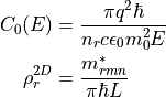
Here,  is the refractive index of the material,
 the reduced,
in-plane, effective mass and
the reduced,
in-plane, effective mass and  an effective period of the
quantum wells. The in-plane effective mass of each type of carriers is
calculated for each level, accounting for the spread of the wavefunction
into the barriers as ([2]):
an effective period of the
quantum wells. The in-plane effective mass of each type of carriers is
calculated for each level, accounting for the spread of the wavefunction
into the barriers as ([2]):
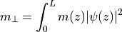
This in-plane effective mass is also used to calculate the local density
of states shown in Figure [fig:qw]b. In Eq. [eq:QW_abs2],
 is the momentum matrix element,
which depends on the polarization of the light and on the Kane’s energy
is the momentum matrix element,
which depends on the polarization of the light and on the Kane’s energy
 , specific to each material and determined experimentally.
For band edge absorption, where
, specific to each material and determined experimentally.
For band edge absorption, where  = 0, the matrix elements for
the absorption of TE and TM polarized light for the transitions
involving the conduction band and the heavy and light holes bands are
given in Table [tab:matrix_elements]. As can be deduced from this
table, transitions involving heavy holes cannot absorb TM polarised
light.
= 0, the matrix elements for
the absorption of TE and TM polarized light for the transitions
involving the conduction band and the heavy and light holes bands are
given in Table [tab:matrix_elements]. As can be deduced from this
table, transitions involving heavy holes cannot absorb TM polarised
light.
TE |
TM |
|
|---|---|---|
|
|
0 |
|
|
|


Table: Momentum matrix elements for transitions in QWs.
 is the bulk matrix element.
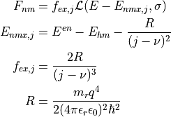
In addition to the band-to-band transitions, QWs usually have strong
excitonic absorption, included in Eq. [eq:qw_abs] in the term
 . This term is a Lorenzian (or Gaussian) defined by an
energy
. This term is a Lorenzian (or Gaussian) defined by an
energy  and oscillator strength
  . It
is zero except for
. It
is zero except for  where it is given by Klipstein
et al. ([3]):
where it is given by Klipstein
et al. ([3]):
Here,  is a constant with a value between 0 and 0.5 and
 is the width of the Lorentzian, both often adjusted to
fit some experimental data. In Solcore, they have default values of
= 0.15 and = 6 meV.
is the width of the Lorentzian, both often adjusted to
fit some experimental data. In Solcore, they have default values of
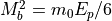
= 0.15 and = 6 meV.  is the exciton
Rydberg energy ([1]).
is the exciton
Rydberg energy ([1]).
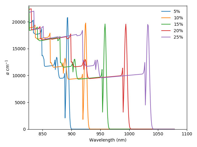
Fig. [fig:QW_absorption] shows the absorption coefficient of a range of InGaAs/GaAsP QWs with a GaAs interlayer and different In content. Higher indium content increases the depth of the well, allowing the absorption of less energetic light and more transitions.