Absorption of quantum wells¶

For modelling the optical properties of QWs we use the method described by S. Chuang ([1]). The absorption coefficient at thermal equilibrium in a QW is given by:

$\label{eq:QW_abs2} \begin{split} \alpha_0(E) & = C_0(E) \sum_{n,m} |I_{hm}^{en}|^2 | \hat{e} \cdot \vec{p} |^2 \rho_{rmn}^{2D} \\ & \times \left[ H(E-E^{en} + E_{hm}) + F_{nm}(E) \right] \end{split}$

where $|I_{hm}^{en}|^2$ is the overlap integral between the holes in level $m$ and the electrons in level $n$ ; $H$ is a step function, $H(x)$ = 1 for $x>0$ , 0 and 0 for $x<0$ , $\rho_{rmn}^{2D}$ is the 2D joint density of states, $C_0$ a proportionality constant dependent on the energy, and $F$ the excitonic contribution, which will be discussed later.

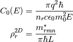
$\begin{aligned} \label{eq:qw_abs} C_0 (E) & = \frac{\pi q^2 \hbar }{n_r c \epsilon_0 m_0^2 E} \\ \rho_r^{2D} &= \frac{m_{rmn}^*}{\pi \hbar L}\end{aligned}$

Here, $n_r$ is the refractive index of the material, $m_{rmn} = m_{en} m_{hm} / (m_{en} + m_{hm})$ the reduced, in-plane, effective mass and $L$ an effective period of the quantum wells. The in-plane effective mass of each type of carriers is calculated for each level, accounting for the spread of the wavefunction into the barriers as ([2]):

$\begin{aligned} \label{eq:in_plane} m_{\perp} = \int_{0}^{L} m(z) | \psi(z) |^2\end{aligned}$

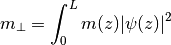
This in-plane effective mass is also used to calculate the local density of states shown in Figure [fig:qw]b. In Eq. [eq:QW_abs2], $| \hat{e} \cdot \vec{p} |^2$ is the momentum matrix element, which depends on the polarization of the light and on the Kane’s energy $E_p$ , specific to each material and determined experimentally. For band edge absorption, where $k$ = 0, the matrix elements for the absorption of TE and TM polarized light for the transitions involving the conduction band and the heavy and light holes bands are given in Table [tab:matrix_elements]. As can be deduced from this table, transitions involving heavy holes cannot absorb TM polarised light.

	TE	TM
$c-hh$	$3/2 M_b^2$	0
$c-lh$	$1/2 M_b^2$	$2 M_b^2$

Table: Momentum matrix elements for transitions in QWs. 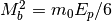$M_b^2=m_0 E_p /6$ is the bulk matrix element.

In addition to the band-to-band transitions, QWs usually have strong excitonic absorption, included in Eq. [eq:qw_abs] in the term $F_{nm}$ . This term is a Lorenzian (or Gaussian) defined by an energy $E_{nmx, j}$ and oscillator strength $f_{ex, j}$ . It is zero except for $m=n \equiv j$ where it is given by Klipstein et al. ([3]):

$\begin{aligned} F_{nm} &= f_{ex, j} \mathcal{L}(E - E_{nmx, j}, \sigma) \\ E_{nmx, j} &= E^{en} - E_{hm} - \frac{R}{(j-\nu)^2} \\ f_{ex, j} &= \frac{2R}{(j-\nu)^3} \\ R &= \frac{m_r q^4}{2 ( 4\pi \epsilon_r \epsilon_0)^2 \hbar^2 }\end{aligned}$

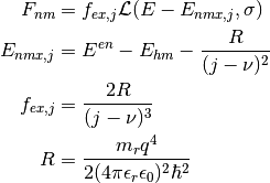
Here, $\nu$ is a constant with a value between 0 and 0.5 and $\sigma$ is the width of the Lorentzian, both often adjusted to fit some experimental data. In Solcore, they have default values of $\nu$ = 0.15 and $\sigma$ = 6 meV. $R$ is the exciton Rydberg energy ([1]).

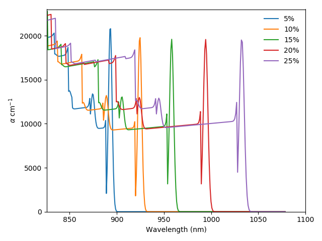
Fig. [fig:QW_absorption] shows the absorption coefficient of a range of InGaAs/GaAsP QWs with a GaAs interlayer and different In content. Higher indium content increases the depth of the well, allowing the absorption of less energetic light and more transitions.

solcore.absorption_calculator.absorption_QW.exciton_rydberg_energy_2d(me, mh, eps_r)[source]¶

Parameters:	me – electron effective mass (units: kg) mh – hole effective mass (units: kg) eps_r – dielectic constant (units: SI)
Returns:	The exciton Rydberg energy

solcore.absorption_calculator.absorption_QW.exciton_bohr_radius(me, mh, eps)[source]¶

Parameters:	me – electron effective mass (units: kg) mh – hole effective mass (units: kg) eps – dielectic constant (units: SI)
Returns:	Exciton Borh radius

solcore.absorption_calculator.absorption_QW.alpha_c_hh_TE(E, z, E_e, E_hh, psi_e, psi_hh, well_width, me, mhh, Ep, nr)[source]¶

Absortion coefficient for incident light forming a transision between hh and c band of a quantum well

NB. Assumes that valence band is a zero energy, might need to manually apply an offset.

Parameters:

E – photon energy (units: J)
z – mesh points along growth direction (units: m)
E_e – Electron state energy (units: J)
E_hh – Heavy hole state energy (units: J)
psi_e – Electron envelope function (psi_e^2 must be normalised)
psi_hh – Heavy hole envelope function (psi_hh^2 must be normalised)
well_width – (units: m)
me – electron effective mass (units: kg)
mhh – heavy hole effective mass (units: kg)
Ep – the Kane parameter “Optical dipole matrix elemet”, sometimes “Momentum matrix element”, e.g. Ep for GaAs ~ 28eV
nr – refractive index

Returns:

solcore.absorption_calculator.absorption_QW.alpha_c_lh_TE(E, z, E_e, E_lh, psi_e, psi_lh, well_width, me, mlh, Ep, nr)[source]¶

Absortion coefficient for incident light forming a transision between hh and c band of a quantum well

NB. Assumes that valence band is a zero energy, might need to manually apply an offset.

Parameters:

E – photon energy (units: J)
z – mesh points along growth direction (units: m)
E_e – Electron state energy (units: J)
E_hh – Heavy hole state energy (units: J)
psi_e – Electron envelope function (psi_e^2 must be normalised)
psi_hh – Heavy hole envelope function (psi_hh^2 must be normalised)
well_width – (units: m)
me – electron effective mass (units: kg)
mhh – heavy hole effective mass (units: kg)
Ep – the Kane parameter “Optical dipole matrix elemet”, sometimes “Momentum matrix element”, e.g. Ep for GaAs ~ 28eV
nr – refractive index

Returns:

solcore.absorption_calculator.absorption_QW.alpha_exciton_ehh_TE(exciton_index, E, z, E_e, E_hh, psi_e, psi_hh, well_width, me, mhh, Ep, nr, eps, hwhm=9.6e-22, dimensionality=0.15, line_shape='Lorenzian')[source]¶

Parameters:	exciton_index – E – z – E_e – E_hh – psi_e – psi_hh – well_width – me – mhh – Ep – nr – eps – hwhm – dimensionality – line_shape –
Returns:

solcore.absorption_calculator.absorption_QW.alpha_exciton_elh_TE(exciton_index, E, z, E_e, E_lh, psi_e, psi_lh, well_width, me, mlh, Ep, nr, eps, hwhm=9.6e-22, dimensionality=0.15, line_shape='Lorenzian')[source]¶

Parameters:	exciton_index – E – z – E_e – E_lh – psi_e – psi_lh – well_width – me – mlh – Ep – nr – eps – hwhm – dimensionality – line_shape –
Returns:

solcore.absorption_calculator.absorption_QW.sum_alpha_c_hh_TE(E, z, E_e, E_hh, psi_e, psi_hh, well_width, me, mh, Ep, nr)[source]¶

Parameters:	E – z – E_e – E_hh – psi_e – psi_hh – well_width – me – mh – Ep – nr –
Returns:

solcore.absorption_calculator.absorption_QW.sum_alpha_c_lh_TE(E, z, E_e, E_lh, psi_e, psi_lh, well_width, me, mh, Ep, nr)[source]¶

Parameters:	E – z – E_e – E_lh – psi_e – psi_lh – well_width – me – mh – Ep – nr –
Returns:

solcore.absorption_calculator.absorption_QW.sum_alpha_exciton_c_hh_TE(E, z, E_e, E_hh, psi_e, psi_hh, well_width, me, mh, Ep, nr, eps, hwhm=9.6e-22, dimensionality=0.5, line_shape='Lorenzian')[source]¶

Parameters:	E – z – E_e – E_hh – psi_e – psi_hh – well_width – me – mh – Ep – nr – eps – hwhm – dimensionality – line_shape –
Returns:

solcore.absorption_calculator.absorption_QW.sum_alpha_exciton_c_lh_TE(E, z, E_e, E_lh, psi_e, psi_lh, well_width, me, mlh, Ep, nr, eps, hwhm=9.6e-22, dimensionality=0.5, line_shape='Lorenzian')[source]¶

Parameters:	E – z – E_e – E_lh – psi_e – psi_lh – well_width – me – mlh – Ep – nr – eps – hwhm – dimensionality – line_shape –
Returns:

solcore.absorption_calculator.absorption_QW.calc_alpha(QM_result, well_width, kane_parameter=4.48e-18, refractive_index=3.5, hwhm=9.6e-22, dimensionality=0.5, theta=0, eps=1.1421902283930001e-10, espace=None, line_shape='Lorenzian')[source]¶

Calculates the absorption coeficient of a quantum well structure assuming the parabolic approximation for the effective masses.

Parameters:

QM_result – The output of the Schrodinger solver, incldued in the ‘quantum_mechanics’ package
well_width – The well width
kane_parameter – The Kane parameter
refractive_index – Refractive (effective) index of the QW
hwhm – Full width at half maximum of the excitonic lineshape
dimensionality –
theta –
eps –
espace –
line_shape –

Returns:

solcore.absorption_calculator.absorption_QW.NonBlackBodyEmission(E, voltage=0, nr=3.5, T=300)[source]¶

Parameters:	E – voltage – nr – T –
Returns:

solcore.absorption_calculator.absorption_QW.calc_emission(QM_result, well_width, voltage=0, theta=0)[source]¶

Parameters:	QM_result – well_width – voltage – theta –
Returns:

References¶

[1]	(1, 2) Chuang, S.L.: Physics of Optoelectronic Devices. Wiley- Interscience, New York (1995)

[2]	Barnham, K., Vvedensky, D. (eds.): Low-Dimensional Semi- conductor Structures: Fundamentals and Device Applications. Cambridge University Press, Cambridge (2001)

[3]	Klipstein, P.C., Apsley, N.: A theory for the electroreflectance spec- tra of quantum well structures. J. Phys. C Solid State Phys. 19(32), 6461–6478 (2000)

Table of Contents

Previous topic

Next topic

This Page

Absorption of quantum wells¶

References¶