from solcore.absorption_calculator.nk_db import download_db, search_db
from solcore import material
from solcore import si
from solcore.solar_cell import SolarCell
from solcore.structure import Layer
from solcore.solar_cell_solver import solar_cell_solver, default_options
import numpy as np
import matplotlib.pyplot as plt
wl = si(np.arange(100, 900, 10), 'nm')
opts = default_options
opts.optics_method = 'TMM'
opts.wavelength = wl
# Download the database from refractiveindex.info. This only needs to be done once.
# Can specify the source URL and number of interpolation points.
# download_db()
# Can search the database to select an appropriate entry. Search by element/chemical formula.
# In this case, look for silver.
search_db('Ag', exact = True)
# This prints out, line by line, matching entries. This shows us entries with
# "pageid"s 0 to 14 correspond to silver.
# Let's compare the optical behaviour of some of those sources:
# pageid = 0, Johnson
# pageid = 2, McPeak
# pageid = 8, Hagemann
# pageid = 12, Rakic (BB)
# create instances of materials with the optical constants from the database.
# The name (when using Solcore's built-in materials, this would just be the
# name of the material or alloy, like 'GaAs') is the pageid, AS A STRING, while
# the flag nk_db must be set to True to tell Solcore to look in the previously
# downloaded database from refractiveindex.info
Ag_Joh = material(name = '0', nk_db=True)()
Ag_McP = material(name = '2', nk_db=True)()
Ag_Hag = material(name = '8', nk_db=True)()
Ag_Rak = material(name = '12', nk_db=True)()
Ag_Sol = material(name = 'Ag')() # Solcore built-in (from SOPRA)
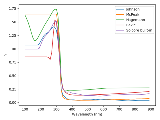
# plot the n and k data. Note that not all the data covers the full wavelength range,
# so the n/k value stays flat.
names = ['Johnson', 'McPeak', 'Hagemann', 'Rakic', 'Solcore built-in']
plt.figure()
plt.plot(wl * 1e9, Ag_Joh.n(wl), wl * 1e9, Ag_McP.n(wl),
wl * 1e9, Ag_Hag.n(wl), wl * 1e9, Ag_Rak.n(wl), wl * 1e9, Ag_Sol.n(wl))
plt.legend(labels=names)
plt.xlabel("Wavelength (nm)")
plt.ylabel("n")
plt.show()
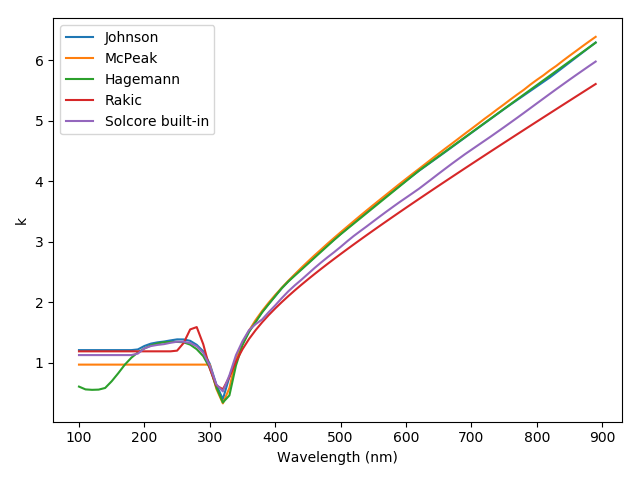
plt.figure()
plt.plot(wl * 1e9, Ag_Joh.k(wl), wl * 1e9, Ag_McP.k(wl),
wl * 1e9, Ag_Hag.k(wl), wl * 1e9, Ag_Rak.k(wl), wl * 1e9, Ag_Sol.k(wl))
plt.legend(labels=names)
plt.xlabel("Wavelength (nm)")
plt.ylabel("k")
plt.show()
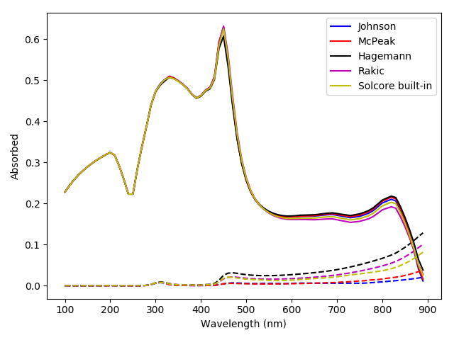
# Compare performance as a back mirror on a GaAs 'cell'
# Solid line: absorption in GaAs
# Dashed line: absorption in Ag
GaAs = material('GaAs')()
colors = ['b', 'r', 'k', 'm', 'y']
plt.figure()
for c, Ag_mat in enumerate([Ag_Joh, Ag_McP, Ag_Hag, Ag_Rak, Ag_Sol]):
my_solar_cell = SolarCell([Layer(width=si('50nm'), material = GaAs)] +
[Layer(width = si('100nm'), material = Ag_mat)])
solar_cell_solver(my_solar_cell, 'optics', opts)
GaAs_positions = np.linspace(my_solar_cell[0].offset, my_solar_cell[0].offset + my_solar_cell[0].width, 1000)
Ag_positions = np.linspace(my_solar_cell[1].offset, my_solar_cell[1].offset + my_solar_cell[1].width, 1000)
GaAs_abs = np.trapz(my_solar_cell[0].diff_absorption(GaAs_positions), GaAs_positions)
Ag_abs = np.trapz(my_solar_cell[1].diff_absorption(Ag_positions), Ag_positions)
plt.plot(wl*1e9, GaAs_abs, color=colors[c], linestyle='-', label=names[c])
plt.plot(wl*1e9, Ag_abs, color=colors[c], linestyle='--')
plt.legend()
plt.xlabel("Wavelength (nm)")
plt.ylabel("Absorbed")
plt.show()