
Radiative coupling in a MJ solar cell
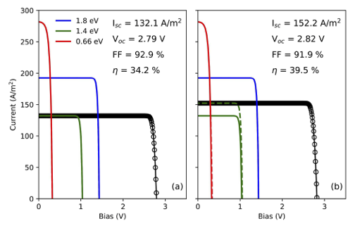
The figure shows the IV curve under the AM1.5G solar
spectrum of a three junction solar cell (a) without and (b) with
radiative coupling. Without coupling, the middle junction severely
limits the current of the MJ solar cell. When coupling is enabled, the
middle junction is still the limiting one but part of the excess current
of the top junction is transferred to it, increasing its photocurrent by
around 20 A/m . Part of the radiative recombination is also
transferred to the bottom cell, increasing slightly its photocurrent. In
this case, given that the junction was overproducing current already,
such coupling is only visible as an increase in the voltage. Altogether,
the radiative coupling results in an enhancement of the V
. Part of the radiative recombination is also
transferred to the bottom cell, increasing slightly its photocurrent. In
this case, given that the junction was overproducing current already,
such coupling is only visible as an increase in the voltage. Altogether,
the radiative coupling results in an enhancement of the V of 30 mV and of the efficiency
  of 5.3%. This example uses
junctions with 100% radiative efficiency to illustrate the effect, but
this phenomenon is always present to some extent, becoming especially
important under concentration.
of 5.3%. This example uses
junctions with 100% radiative efficiency to illustrate the effect, but
this phenomenon is always present to some extent, becoming especially
important under concentration.
import matplotlib.pyplot as plt
import numpy as np

from solcore.structure import Junction
from solcore.solar_cell import SolarCell
from solcore.light_source import LightSource
from solcore.solar_cell_solver import solar_cell_solver
from solcore.graphing.Custom_Colours import colours

T = 298

Vin = np.linspace(-6, 2, 600)
V = np.linspace(-1.5, 4, 500)
wl = np.linspace(350, 2000, 301) * 1e-9
light_source = LightSource(source_type='standard', version='AM1.5g', x=wl, output_units='photon_flux_per_m',
                           concentration=1)

color = ['b', 'g', 'r']
label = ['Top', 'Mid', 'Bot']

fig, ax = plt.subplots(1, 2, sharey='all', figsize=(7, 4.5))

for k, rad in enumerate([False, True]):

    # Input data for the 2D kind of junction
    db_junction = Junction(kind='2D', T=T, reff=0.3, jref=300, Eg=0.66, A=1, R_shunt=np.inf, n=3.5)
    db_junction2 = Junction(kind='2D', T=T, reff=1, jref=300, Eg=1.4, A=1, R_shunt=np.inf, n=3.5)
    db_junction3 = Junction(kind='2D', T=T, reff=1, jref=300, Eg=1.8, A=1, R_shunt=np.inf, n=3.5)

    my_solar_cell = SolarCell([db_junction3, db_junction2, db_junction], T=T, R_series=0)

    solar_cell_solver(my_solar_cell, 'iv',
                      user_options={'T_ambient': T, 'voltages': V, 'light_iv': True, 'wavelength': wl,
                                    'light_source': light_source, 'radiative_coupling': rad, 'mpp': True,
                                    'internal_voltages': Vin})

    # This is the total junction IV
    ax[k].plot(my_solar_cell.iv['IV'][0], my_solar_cell.iv['IV'][1], marker='o', color=colours("Black"), ls='-',
               markerfacecolor='none', markeredgecolor=colours("Black"))

    # This is the junciton IV when it is in the MJ device, including coupling if it is enabled.
    for i, data in enumerate(my_solar_cell.iv['junction IV']):
        ax[k].plot(data[0], data[1], color[i] + '--', linewidth=2)

    # This is the junction IV as if it were an isolated device and therefore not affected by coupling or current limiting.
    for i in range(my_solar_cell.junctions):
        ax[k].plot(V, -my_solar_cell(i).iv(V), color[i], linewidth=2, label=label[i])

    ax[k].set_ylim(0, 300)
    ax[k].set_xlim(0, 3.5)

    ax[k].set_xlabel('Bias (V)')

    Isc = my_solar_cell.iv["Isc"]
    Voc = my_solar_cell.iv["Voc"]
    FF = my_solar_cell.iv["FF"] * 100
    Eta = my_solar_cell.iv["Eta"] * 100

    ax[k].text(1.75, 275, 'I$_{sc}$ = ' + str(round(Isc, 1)) + ' A/m$^2$', fontsize=12)
    ax[k].text(1.75, 250, 'V$_{oc}$ = ' + str(round(Voc, 2)) + ' V', fontsize=12)
    ax[k].text(1.75, 225, 'FF = {:.1f} %'.format(FF), fontsize=12)
    ax[k].text(1.75, 200, r'$\eta$ = {:.1f} %'.format(Eta), fontsize=12)

ax[0].set_ylabel('Current (A/m$^2$)')
ax[0].text(0.9, 0.05, '(a)', transform=ax[0].transAxes, fontsize=12)
ax[1].text(0.9, 0.05, '(b)', transform=ax[1].transAxes, fontsize=12)
plt.tight_layout()
ax[0].legend(loc=(0.10, 0.80), frameon=False)
plt.show()