import numpy as np
import matplotlib.pyplot as plt
from solcore import material
from solcore.constants import electron_mass
from solcore.quantum_mechanics import kp_bands
# Material parameters
GaAs = material("GaAs")(T=300)
InGaAs = material("InGaAs")
# As a test, we solve the problem for an intermediate indium composition
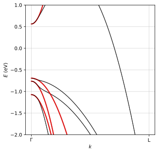
InGaAs2 = InGaAs(In=0.15, T=300)
masses = kp_bands(InGaAs2, GaAs, graph=True, fit_effective_mass=True, effective_mass_direction="L", return_so=True)
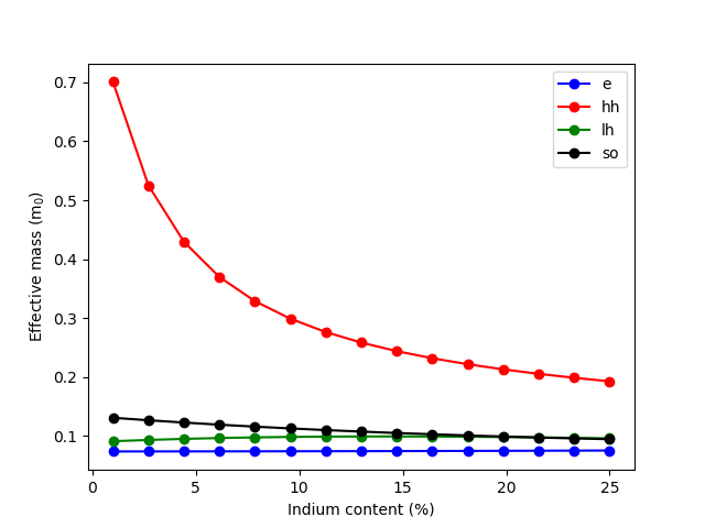
comp = np.linspace(0.01, 0.25, 15)
me = []
mhh = []
mlh = []
mso = []
for i in comp:
InGaAs2 = InGaAs(In=i, T=300)
# Set graph = True to see the fitting of the bands
c, hh, lh, so, m_eff_c, m_eff_hh, m_eff_lh, m_eff_so = kp_bands(InGaAs2, GaAs, graph=False, fit_effective_mass=True,
effective_mass_direction="L", return_so=True)
me.append(m_eff_c / electron_mass)
mhh.append(m_eff_hh / electron_mass)
mlh.append(m_eff_lh / electron_mass)
mso.append(m_eff_so / electron_mass)
print('Effective masses for In = {:2.3}%:'.format(i * 100))
print('- m_e = {:1.3f} m0'.format(me[-1]))
print('- m_hh = {:1.3f} m0'.format(mhh[-1]))
print('- m_lh = {:1.3f} m0'.format(mlh[-1]))
print('- m_so = {:1.3f} m0'.format(mso[-1]))
print()
plt.plot(comp * 100, me, 'b-o', label='e')
plt.plot(comp * 100, mhh, 'r-o', label='hh')
plt.plot(comp * 100, mlh, 'g-o', label='lh')
plt.plot(comp * 100, mso, 'k-o', label='so')
plt.xlabel("Indium content (%)")
plt.ylabel("Effective mass (m$_0$)")
plt.legend()
plt.show()