Optical properties of materials
Solcore has several ways of accessing the optical properties of materials: databases and parametric dielectric functions.
Dielectric constants models and Adachi parametrization
Understanding the optical response of both established and novel
materials is crucial to effective solar cell design. To efficiently
model the complex dielectric function of a material Solcore incorporates
an optical constant calculator based on the well-known Critical-Point
Parabolic-Band (CPPB) formalism popularised by Adachi ([1], [2], [3]). In this
model, contributions to :math:`epsilon_2(omega)` from critical
points in the Brillouin Zone at which the probability for optical
transitions is large (van Hove singularities) are considered. The
transition probability for such transitions is proportional to the joint
density of states (JDOS)  , which
describes the number of available electronic states between the valence
and conduction bands at given photon energy. The imaginary part of the
complex dielectric function is related to the JDOS by:
, which
describes the number of available electronic states between the valence
and conduction bands at given photon energy. The imaginary part of the
complex dielectric function is related to the JDOS by:
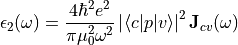
Where  is
the momentum matrix element for transitions from the valence band
(
is
the momentum matrix element for transitions from the valence band
( ) to the conduction band (
 ). Critical point
transitions are considered at the following points of symmetry in the
band structure: :math:`E_0` corresponds to the optical transition at
the :math:`Gamma` point and :math:`E_0 + Delta_0` to the
transition from the spin-orbit split off band to the conduction band at
the :math:`Gamma` point. :math:`E_1` and :math:`E_1 + Delta_1`
denote the transitions from the valence heavy-hole (HH) band and the
valence light-hole (LH) band respectively to the conduction band at the
L point. The :math:`E’_0` triplet and :math:`E_2` transitions
occur at higher energies, between the HH band and the split conduction
bands at the
). Critical point
transitions are considered at the following points of symmetry in the
band structure: :math:`E_0` corresponds to the optical transition at
the :math:`Gamma` point and :math:`E_0 + Delta_0` to the
transition from the spin-orbit split off band to the conduction band at
the :math:`Gamma` point. :math:`E_1` and :math:`E_1 + Delta_1`
denote the transitions from the valence heavy-hole (HH) band and the
valence light-hole (LH) band respectively to the conduction band at the
L point. The :math:`E’_0` triplet and :math:`E_2` transitions
occur at higher energies, between the HH band and the split conduction
bands at the  point as well as across the wide gap X
valley. The model also includes contributions from the lowest energy
indirect band-gap transition and the exciton absorption at the
:math:`E_0` critical point. The contributions listed above are summed
to compute the overall value of
point as well as across the wide gap X
valley. The model also includes contributions from the lowest energy
indirect band-gap transition and the exciton absorption at the
:math:`E_0` critical point. The contributions listed above are summed
to compute the overall value of  . The real and
imaginary components of the overall complex dielectric function
. The real and
imaginary components of the overall complex dielectric function
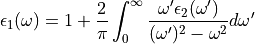
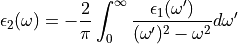
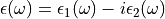 are
then related via the Kramers-Kronig relations;
are
then related via the Kramers-Kronig relations;
The CPPB model included with Solcore also incorporates a modification to
the critical point broadening present in Adachi’s description, which is
shown to produce a poor fit to experimental data in the vicinity of the
 and
and  critical points ([4]). To give a more accurate description of
the broadening of the optical dielectric function, Kim et al. proposed
that a frequency-dependent damping parameter be used to replace the
damping constant given by Adachi at each critical point
([5], [6]);
critical points ([4]). To give a more accurate description of
the broadening of the optical dielectric function, Kim et al. proposed
that a frequency-dependent damping parameter be used to replace the
damping constant given by Adachi at each critical point
([5], [6]);
![\label{eqn:Kim_damping}
\Gamma'(\omega) = \Gamma exp \left[ -\alpha \left( \frac{\hbar \omega - E_0}{\Gamma}\right) ^2 \right]](../_images/math/44345e7a0fbd7a39557d7bc1a292285784c01156.png)
Where is the damping constant used by Adachi and
 describes the shape of the lineshape broadening with
 producing purely Lorentzian character and
 producing a good approximation to Gaussian
broadening.
producing a good approximation to Gaussian
broadening.
The Solcore module absorption_calculator contains the CPPB model
within the Custom_CPPB class. The class offers a flexible way to
build up the optical constant model by adding individual critical point
contributions through the Oscillator structure type within Solcore. In
addition to the oscillator functions described by Adachi the
Custom_CPPB class also provides additional oscilator models and the
Sellmeier equation for describing the real part of the dielectric
function for non-absorbing materials ([7]).
Description of functions in this module
SOPRA database
n order to calculate and model the optical response of potential solar
cell architectures and material systems, access to a library of accurate
optical constant data is essential. Therefore, Solcore incorporates a
resource of freely available optical constant data measured by Sopra S.
A. and provided by Software Spectra Inc.
The refractive index  and
extinction coefficient
and
extinction coefficient  are provided for over 200 materials,
including many III-V, II-VI and group IV compounds in addition to a
range of common metals, glasses and dielectrics.
are provided for over 200 materials,
including many III-V, II-VI and group IV compounds in addition to a
range of common metals, glasses and dielectrics.
Any material within the Sopra S.A. optical constant database can be
used with the “material” function, but they will have
only the optical parameters and . In the case of
materials that are in both databases, the keyword “sopra” will need to
be set to “True” when creating the material. Once a material is loaded
its , and absorption coefficient data is returned by
calling the appropriate method, for example SiO2.n(wavelength) and
SiO2.k(wavelength). For certain materials in the database, the
optical constants are provided for a range of alloy compositions. In
these cases, any desired composition within the range can be specified
and the interpolated and data is returned.
Manually changing optical constants of a material
If you would like to define a material with optical constant data from a file, you can do this by telling Solcore the path to the optical constant data, e.g.:
this_dir = os.path.split(__file__)[0]

SiGeSn = material('Ge')(T=T, electron_mobility=0.05, hole_mobility=3.4e-3)

SiGeSn.n_path = this_dir + '/SiGeSn_n.txt'
SiGeSn.k_path = this_dir + '/SiGeSn_k.txt'
In this case, we have defined a material which is like the built-in Solcore germanium material, but with new data for the refractive index and extinction coefficient from the files SiGeSn_n.txt and SiGeSn_k.txt, respectively, which are in the same folder as the Python script. The format of these files is tab-separated, with the first column being wavelength (in nm) and the second column n or k.