Example of a quasi-3D modelling of a 3J solar cell
(code shown for 1J, but the extension is immediate)
Required extra files, available in Solcore’s Github repository (Examples folder):
masks_illumination.png
masks_sq.png
masks_cl.png
import numpy as np
import matplotlib.pyplot as plt
from solcore.structure import Junction
from solcore.solar_cell import SolarCell
from solcore.light_source import LightSource
from solcore.spice import solve_quasi_3D
# First we load the masks defining the illumination pattern and the contacts. Both must be greyscale images
# The solver expect images with values between 0 and 255 and imread of a PNG image is between 0 and 1, even when
# it is in grey, so we scale it multiplying by 255. If the image were JPG, the result would be already in (0,255).
illuminationMask = (plt.imread('masks_illumination.png') * 255).astype(np.int)
contactsMask = (plt.imread('masks_sq.png') * 255).astype(np.int)
nx, ny = illuminationMask.shape
# For symmetry arguments (not completely true for the illumination), we can mode just 1/4 of the device and then
# multiply the current by 4
illuminationMask = illuminationMask[int(nx / 2):, int(ny / 2):]
contactsMask = contactsMask[int(nx / 2):, int(ny / 2):]
# Size of the pixels (m)
Lx = 10e-6
Ly = 10e-6
# Height of the metal fingers (m)
h = 2.2e-6
# Contact resistance (Ohm m2)
Rcontact = 3e-10
# Resistivity metal fingers (Ohm m)
Rline = 2e-8
# Bias (V)
vini = 0
vfin = 1.3
step = 0.01
T = 298
db_junction = Junction(kind='2D', T=T, reff=1, jref=300, Eg=0.66, A=1, R_sheet_top=100, R_sheet_bot=1e-16,
R_shunt=1e16, n=3.5)
db_junction2 = Junction(kind='2D', T=T, reff=1, jref=300, Eg=1.4, A=1, R_sheet_top=100, R_sheet_bot=1e-16,
R_shunt=1e16, n=3.5)
db_junction3 = Junction(kind='2D', T=T, reff=0.5, jref=300, Eg=1.8, A=1, R_sheet_top=100, R_sheet_bot=100,
R_shunt=1e16, n=3.5)
# For a single junction, this will have >28800 nodes and for the full 3J it will be >86400, so it is worth to
# exploit symmetries whenever possible. A smaller number of nodes also makes the solver more robust.
my_solar_cell = SolarCell([db_junction2], T=T)
wl = np.linspace(350, 2000, 301) * 1e-9
light_source = LightSource(source_type='standard', version='AM1.5g', x=wl, output_units='photon_flux_per_m',
concentration=100)
options = {'light_iv': True, 'wavelength': wl, 'light_source': light_source}
V, I, Vall, Vmet = solve_quasi_3D(my_solar_cell, illuminationMask, contactsMask, options=options, Lx=Lx, Ly=Ly, h=h,
R_back=1e-16, R_contact=Rcontact, R_line=Rline, bias_start=vini, bias_end=vfin,
bias_step=step)
# Since we model 1/4 of the device, we multiply the current by 4
I = I * 4
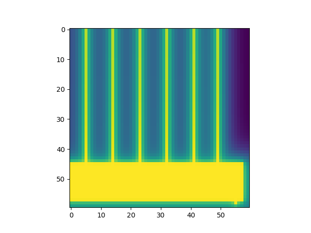
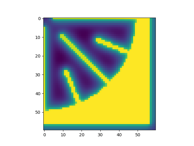
# This will plot the voltage at the last external voltage point V=1.3 V for the top layer of the top junction.
plt.figure(1)
plt.imshow(Vall[:, :, -2, -1])
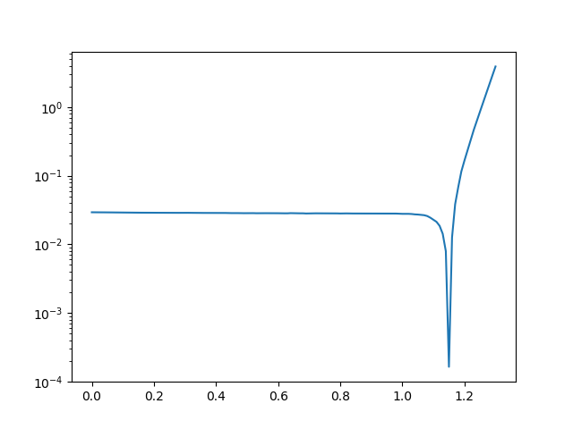
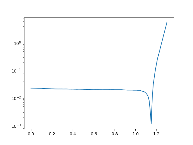
plt.figure(2)
plt.semilogy(V, abs(I))
plt.show()