Example of a 2J solar cell calculated with the PDD solver

import matplotlib.pyplot as plt
import numpy as np

from solcore.solar_cell import SolarCell, default_GaAs
from solcore.structure import Layer, Junction
from solcore import si
from solcore import material
from solcore.light_source import LightSource
from solcore.solar_cell_solver import solar_cell_solver

T = 298

substrate = material('GaAs')(T=T)


def AlGaAs(T):
    # We create the other materials we need for the device
    window = material('AlGaAs')(T=T, Na=5e24, Al=0.8)
    p_AlGaAs = material('AlGaAs')(T=T, Na=1e24, Al=0.4)
    n_AlGaAs = material('AlGaAs')(T=T, Nd=8e22, Al=0.4)
    bsf = material('AlGaAs')(T=T, Nd=2e24, Al=0.6)

    output = Junction([Layer(width=si('30nm'), material=window, role="Window"),
                       Layer(width=si('150nm'), material=p_AlGaAs, role="Emitter"),
                       Layer(width=si('1000nm'), material=n_AlGaAs, role="Base"),
                       Layer(width=si('200nm'), material=bsf, role="BSF")], sn=1e6, sp=1e6, T=T, kind='PDD')

    return output


my_solar_cell = SolarCell([AlGaAs(T), default_GaAs(T)], T=T, R_series=0, substrate=substrate)

Vin = np.linspace(-2, 2.61, 201)
V = np.linspace(0, 2.6, 300)
wl = np.linspace(350, 1000, 301) * 1e-9
light_source = LightSource(source_type='standard', version='AM1.5g', x=wl, output_units='photon_flux_per_m',
                           concentration=1)

# We calculate the IV curve under illumination
solar_cell_solver(my_solar_cell, 'iv',
                  user_options={'T_ambient': T, 'db_mode': 'boltzmann', 'voltages': V, 'light_iv': True,
                                'wavelength': wl, 'optics_method': 'BL', 'mpp': True, 'internal_voltages': Vin,
                                'light_source': light_source})

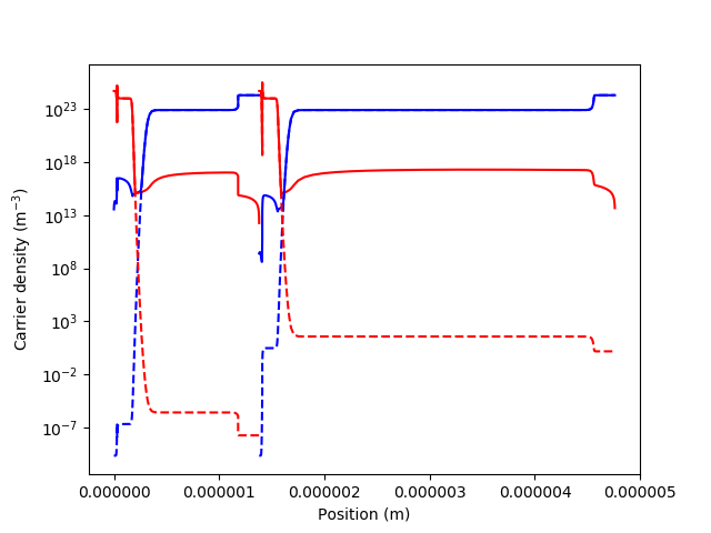
# We can plot the electron and hole densities in equilibrium and at short circuit, both calculated automatically
# before calculating the IV curve
plt.figure(1)
for j in my_solar_cell.junction_indices:
    zz = my_solar_cell[j].short_circuit_data.Bandstructure['x'] + my_solar_cell[j].offset
    n = my_solar_cell[j].short_circuit_data.Bandstructure['n']
    p = my_solar_cell[j].short_circuit_data.Bandstructure['p']
    plt.semilogy(zz, n, 'b')
    plt.semilogy(zz, p, 'r')

    zz = my_solar_cell[j].equilibrium_data.Bandstructure['x'] + my_solar_cell[j].offset
    n = my_solar_cell[j].equilibrium_data.Bandstructure['n']
    p = my_solar_cell[j].equilibrium_data.Bandstructure['p']
    plt.semilogy(zz, n, 'b--')
    plt.semilogy(zz, p, 'r--')

plt.xlabel('Position (m)')
plt.ylabel('Carrier density (m$^{-3}$)')

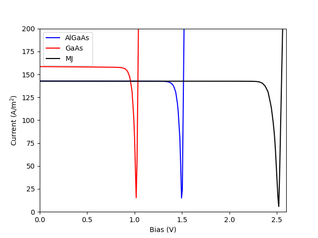
# And the IV curves of the individual junctions and of the MJ device
plt.figure(2)
plt.plot(V, abs(my_solar_cell[0].iv(V)), 'b', label='AlGaAs')
plt.plot(V, abs(my_solar_cell[1].iv(V)), 'r', label='GaAs')
plt.plot(my_solar_cell.iv.IV[0], abs(my_solar_cell.iv.IV[1]), 'k', label='MJ')

plt.legend()
plt.xlim(0, 2.6)
plt.ylim(0, 200)
plt.xlabel('Bias (V)')
plt.ylabel('Current (A/m$^2}$)')

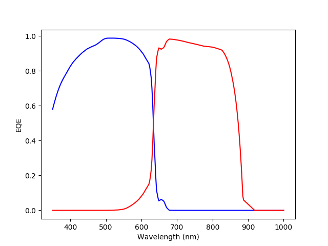
# Now we calculate the quantum efficiency
solar_cell_solver(my_solar_cell, 'qe',
                  user_options={'T_ambient': T, 'db_mode': 'boltzmann', 'voltages': V, 'light_iv': True,
                                'wavelength': wl, 'optics_method': 'BL', 'mpp': True, 'internal_voltages': Vin,
                                'light_source': light_source})

plt.figure(3)

plt.plot(wl * 1e9, my_solar_cell[0].eqe(wl), 'b', label='AlGaAs')
plt.plot(wl * 1e9, my_solar_cell[1].eqe(wl), 'r', label='GaAs')

plt.xlabel('Wavelength (nm)')
plt.ylabel('EQE')

plt.show()