import numpy as np
import matplotlib.pyplot as plt
from matplotlib import cm
from solcore.light_source import LightSource
from solcore.solar_cell import SolarCell
from solcore.solar_cell_solver import solar_cell_solver
from solcore.structure import Junction
# Illumination spectrum
wl = np.linspace(300, 4000, 4000) * 1e-9
light = LightSource(source_type='standard', version='AM1.5g', x=wl, output_units='photon_flux_per_m')
T = 298
V = np.linspace(0, 5, 500)
# This function assembles the solar cell and calculates the IV cruve
def solve_MJ(EgBot, EgMid, EgTop):
db_junction0 = Junction(kind='DB', T=T, Eg=EgBot, A=1, R_shunt=np.inf, n=1)
db_junction1 = Junction(kind='DB', T=T, Eg=EgMid, A=1, R_shunt=np.inf, n=1)
db_junction2 = Junction(kind='DB', T=T, Eg=EgTop, A=1, R_shunt=np.inf, n=1)
# n is the ideality factor of the diode. It is 1 for a perfect diode, but can be higher for a real diode.
my_solar_cell = SolarCell([db_junction2, db_junction1, db_junction0], T=T, R_series=0)
solar_cell_solver(my_solar_cell, 'iv',
user_options={'T_ambient': T, 'db_mode': 'top_hat', 'voltages': V, 'light_iv': True,
'internal_voltages': np.linspace(-6, 5, 1100), 'wavelength': wl,
'mpp': True, 'light_source': light})
return my_solar_cell
# We create an efficiency map using Eg0 as the bandgap of the bottom junction and scanning the bandgaps of the middle
# and top junctions
N1 = 30
N2 = 30
Eg0 = 1.12
all_Eg1 = np.linspace(1.3, 1.8, N1)
all_Eg2 = np.linspace(1.7, 2.4, N2)
eff = np.zeros((N1, N2))
N = N1 * N2
index = 0
Effmax = -1
Eg1_max = all_Eg1[0]
Eg2_max = all_Eg2[0]
# And we run the calculation
for i, Eg1 in enumerate(all_Eg1):
for j, Eg2 in enumerate(all_Eg2):
my_solar_cell = solve_MJ(Eg0, Eg1, Eg2)
mpp = my_solar_cell.iv.Pmpp
eff[i, j] = mpp
if mpp > Effmax:
Effmax = mpp
Eg1_max = Eg1
Eg2_max = Eg2
index += 1
print(int(index / N * 100), '%\n')
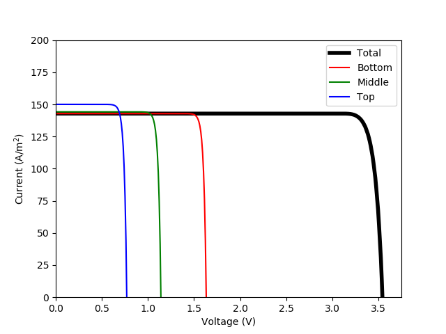
optimum_MJ = solve_MJ(Eg0, Eg1_max, Eg2_max)
plt.figure(1)
plt.plot(V, optimum_MJ.iv.IV[1], 'k', linewidth=4, label='Total')
plt.plot(V, -optimum_MJ[0].iv(V), 'r', label='Bottom')
plt.plot(V, -optimum_MJ[1].iv(V), 'g', label='Middle')
plt.plot(V, -optimum_MJ[2].iv(V), 'b', label='Top')
plt.ylim(0, 200)
plt.xlim(0, 3.75)
plt.legend()
plt.xlabel('Voltage (V)')
plt.ylabel('Current (A/m$^2$)')
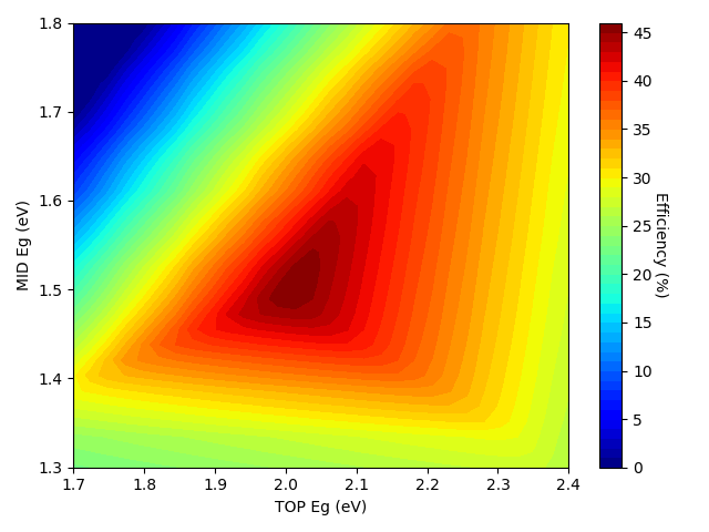
plt.figure(2)
eff = eff / light.power_density * 100
plt.contourf(all_Eg2, all_Eg1, eff, 50, cmap=cm.jet)
plt.xlabel('TOP Eg (eV)')
plt.ylabel('MID Eg (eV)')
cbar = plt.colorbar()
cbar.set_label('Efficiency (%)', rotation=270, labelpad=10)
plt.tight_layout()
plt.show()