import numpy as np
import matplotlib.pyplot as plt
from solcore import siUnits, material, si
from solcore.solar_cell import SolarCell
from solcore.structure import Junction, Layer
from solcore.solar_cell_solver import solar_cell_solver
from solcore.light_source import LightSource
# Define materials for the anti-reflection coating:
MgF2 = material("MgF2")()
ZnS = material("ZnScub")()
ARC_layers = [Layer(si("100nm"), material=MgF2),
Layer(si("50nm"), material=ZnS)]
# TOP CELL - InGaP
# Now we build the top cell, which requires the n and p sides of GaInP and a window
# layer. We also add some extra parameters needed for the calculation using the
# depletion approximation: the minority carriers diffusion lengths and the doping.
AlInP = material("AlInP")
InGaP = material("GaInP")
window_material = AlInP(Al=0.52)
top_cell_n_material = InGaP(In=0.49, Nd=siUnits(2e18, "cm-3"),
hole_diffusion_length=si("200nm"))
top_cell_p_material = InGaP(In=0.49, Na=siUnits(1e17, "cm-3"),
electron_diffusion_length=si("2um"))
# MID CELL - GaAs
GaAs = material("GaAs")
mid_cell_n_material = GaAs(In=0.01, Nd=siUnits(3e18, "cm-3"),
hole_diffusion_length=si("500nm"))
mid_cell_p_material = GaAs(In=0.01, Na=siUnits(1e17, "cm-3"),
electron_diffusion_length=si("5um"))
# BOTTOM CELL - Ge
Ge = material("Ge")
bot_cell_n_material = Ge(Nd=siUnits(2e18, "cm-3"),
hole_diffusion_length=si("800nm"))
bot_cell_p_material = Ge(Na=siUnits(1e17, "cm-3"),
electron_diffusion_length=si("50um"))
# Now that the layers are configured, we can now assemble the triple junction solar
# cell. Note that we also specify a metal shading of 2% and a cell area of $1cm^{2}$.
# SolCore calculates the EQE for all three junctions and light-IV showing the relative
# contribution of each sub-cell. We set "kind = 'DA'" to use the depletion
# approximation. We can also set the surface recombination velocities, where sn
# refers to the surface recombination velocity at the n-type surface, and sp refers
# to the SRV on the p-type side.
solar_cell = SolarCell(
ARC_layers +
[
Junction([Layer(si("25nm"), material=window_material, role='window'),
Layer(si("100nm"), material=top_cell_n_material, role='emitter'),
Layer(si("400nm"), material=top_cell_p_material, role='base'),
], sn=si("1e5cm s-1"), sp=si("1e5cm s-1"), kind='DA'),
Junction([Layer(si("200nm"), material=mid_cell_n_material, role='emitter'),
Layer(si("3000nm"), material=mid_cell_p_material, role='base'),
], sn=si("1e5cm s-1"), sp=si("1e5cm s-1"), kind='DA'),
Junction([Layer(si("400nm"), material=bot_cell_n_material, role='emitter'),
Layer(si("100um"), material=bot_cell_p_material, role='base'),
], sn=si("1e5cm s-1"), sp=si("1e5cm s-1"), kind='DA')
],
shading=0.02, cell_area=1 * 1 / 1e4)
# Choose wavelength range (in m):
wl = np.linspace(280, 1850, 700) * 1e-9
# Calculate the EQE for the solar cell:
solar_cell_solver(solar_cell, 'qe', user_options={'wavelength': wl,
'da_mode': 'green',
'optics_method': 'TMM'
})
# we pass options to use the TMM optical method to calculate realistic R, A and T
# values with interference in the ARC (and semiconductor) layers. We can also choose
# which solver mode to use for the depletion approximation. The default is 'green',
# which uses the (faster) Green's function method. The other method is 'bvp'.
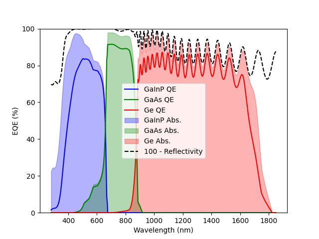
# Plot the EQE and absorption of the individual junctions. Note that we can access
# the properties of the first junction (ignoring any other layers, such as the ARC,
# which are not part of a junction) using solar_cell(0), and the second junction using
# solar_cell(1), etc.
plt.figure(1)
plt.plot(wl * 1e9, solar_cell(0).eqe(wl) * 100, 'b', label='GaInP QE')
plt.plot(wl * 1e9, solar_cell(1).eqe(wl) * 100, 'g', label='GaAs QE')
plt.plot(wl * 1e9, solar_cell(2).eqe(wl) * 100, 'r', label='Ge QE')
plt.fill_between(wl * 1e9, solar_cell(0).layer_absorption * 100, 0, alpha=0.3,
label='GaInP Abs.', color='b')
plt.fill_between(wl * 1e9, solar_cell(1).layer_absorption * 100, 0, alpha=0.3,
label='GaAs Abs.', color='g')
plt.fill_between(wl * 1e9, solar_cell(2).layer_absorption * 100, 0, alpha=0.3,
label='Ge Abs.', color='r')
plt.plot(wl*1e9, 100*(1-solar_cell.reflected), '--k', label="100 - Reflectivity")
plt.legend()
plt.ylim(0, 100)
plt.ylabel('EQE (%)')
plt.xlabel('Wavelength (nm)')
plt.show()
# Set up the AM0 (space) solar spectrum for the light I-V calculation:
am0 = LightSource(source_type='standard',version='AM0',x=wl,
output_units='photon_flux_per_m')
# Set up the voltage range for the overall cell (at which the total I-V will be
# calculated) as well as the internal voltages which are used to calculate the results
# for the individual junctions. The range of the internal_voltages should generally
# be wider than that for the voltages.
# this is an n-p cell, so we need to scan negative voltages
V = np.linspace(-3, 0, 300)
internal_voltages = np.linspace(-4, 2, 400)
# Calculate the current-voltage relationship under illumination:
solar_cell_solver(solar_cell, 'iv', user_options={'light_source': am0,
'voltages': V,
'internal_voltages': internal_voltages,
'light_iv': True,
'wavelength': wl,
'optics_method': 'TMM',
'mpp': True,
})
# We pass the same options as for solving the EQE, but also set 'light_iv' and 'mpp' to
# True to indicate we want the IV curve under illumination and to find the maximum
# power point (MPP). We also pass the AM0 light source and voltages created above.
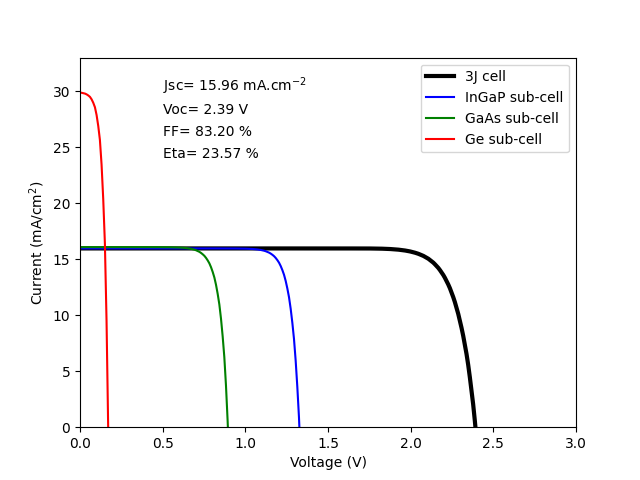
plt.figure(2)
plt.plot(abs(V), -solar_cell.iv['IV'][1]/10, 'k', linewidth=3, label='3J cell')
plt.plot(abs(V), solar_cell(0).iv(V)/10, 'b', label='InGaP sub-cell')
plt.plot(abs(V), solar_cell(1).iv(V)/10, 'g', label='GaAs sub-cell')
plt.plot(abs(V), solar_cell(2).iv(V)/10, 'r', label='Ge sub-cell')
plt.text(0.5,30,f'Jsc= {abs(solar_cell.iv.Isc/10):.2f} mA.cm' + r'$^{-2}$')
plt.text(0.5,28,f'Voc= {abs(solar_cell.iv.Voc):.2f} V')
plt.text(0.5,26,f'FF= {solar_cell.iv.FF*100:.2f} %')
plt.text(0.5,24,f'Eta= {solar_cell.iv.Eta*100:.2f} %')
plt.legend()
plt.ylim(0, 33)
plt.xlim(0, 3)
plt.ylabel('Current (mA/cm$^2$)')
plt.xlabel('Voltage (V)')
plt.show()